In the Buckley lab, we have been using a MacGuyvered sequence analysis pipeline with components from Mothur, QIIME, and custom scripts for the majority of our amplicon sequence datasets. Before leaving for a new position, Chuck Pepe-Ranney (a previous postdoc in the Buckley lab) introduced me to the DADA2 pipeline and laid the groundwork for our lab’s transition to use it. I have since been working with fellow labmates to integrate DADA2 into our analytical pipeline and wanted to share how we’re using it today.

This tutorial will walk through the basic steps needed to process 16S rRNA amplicon datasets using the DADA2 package in R. It is basically a rehashing of what is presented here with some minor changes and a few additional steps for easy handoff to existing scripts we use.

Data Formatting

DADA2 expects a certain file format before running. For each sample, there should be two fastq files - one with all read 1 sequences, and one with all read 2 sequences. Files should be named with the format SAMPLE.R1.fastq. Normally you can ask for sequences to be returned to you in this format from your sequencing center, or use a custom demultiplexing script to generate these sequences from multiplexed files.

Quality Control and Sequence Binning with DADA2 Miltithreading Pipeline

Check Sequence Quality

First, we need to check the quality of our sequences in order to determine our cutoffs and filtering criteria. To do this we will plot the quality scores of our samples as shown below.

library(dada2)
# Prepare file names for DADA2 pipeline

path  = "demo_seqs/"
fns = list.files(path)

fastqs = fns[grepl(".fq.gz$", fns)]
fastqs = sort(fastqs) # Sort ensures forward/reverse reads are in same order
fnFs = fastqs[grepl("R1", fastqs)] # Just the forward read files
fnRs = fastqs[grepl("R2", fastqs)] # Just the reverse read files

# Get sample names from the first part of the forward read filenames
sample_names = sapply(strsplit(fnFs, "[.]"), `[`, 1)

# Fully specify the path for the fnFs and fnRs
fnFs <- paste0(path, fnFs)
fnRs <- paste0(path, fnRs)

# Plot quality profile for each sample. Change the number in brackets to look at a different sample's profile.
plotQualityProfile(fnFs[[1]])

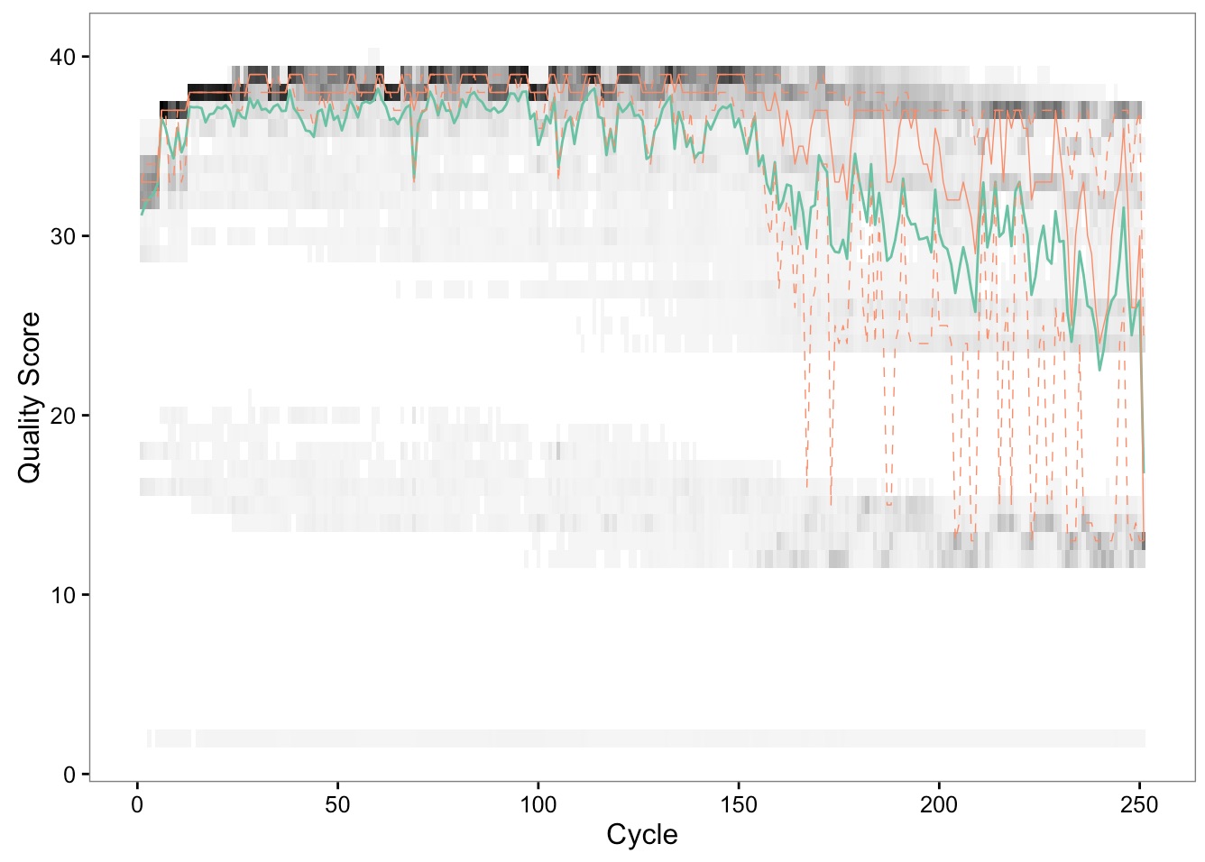
We can see from this plot that our sequences start to drop in quality around base 150. Additionally, the first 10 bases are lower quality than the rest. You should repeat this for the reverse reads, and use these cutoffs in the code chunk below.

Note: Oddly, if you attempt to run the next blocks of code in the same instance of R that you ran the previous block of code, we have seen odd stalling/errors arise. I would recommend that at this point you restart your R session and proceed.

Filter Sequences

Next, we will run filtering on all samples. Previously, a cutoff of 150 bases for each forward and reverse read was determined. This cutoff is the norm for sequences generated at the Cornell sequencing center.

filtFs = paste0(path, sample_names, "_F_filt.fastq.gz")
filtRs = paste0(path, sample_names, "_R_filt.fastq.gz")

if(length(fnFs) != length(fnRs)) stop("Forward and reverse files do not match.")
# Filtering: THESE PARAMETERS ARENT OPTIMAL FOR ALL DATASETS. Trim sequences based on quality profile from raw fastq files. 
for(i in seq_along(fnFs)) {
  fastqPairedFilter(c(fnFs[i], fnRs[i]), c(filtFs[i], filtRs[i]),
                    trimLeft=c(10, 10), truncLen=c(150,150), 
                    maxN=0, maxEE=2, truncQ=2, 
                    compress=TRUE, verbose=TRUE)
}

Run Sample Inference

This code chuck dereplicates our sequences (trims down to only unique sequences while maintaning an average quality score profile) and performs the core algorithm of DADA2. At the end, a final sequence table is made and chimeras are removed.

#Set sample names based on file names.
sample.names <- sapply(strsplit(basename(filtFs), "_"), `[`, 1)
names(filtFs) <- sample.names
names(filtRs) <- sample.names
set.seed(100)
# Learn forward error rates
NSAM.LEARN <- 25 # Choose enough samples to have at least 1M reads
drp.learnF <- derepFastq(sample(filtFs, NSAM.LEARN))
dd.learnF <- dada(drp.learnF, err=NULL, selfConsist=TRUE, multithread=TRUE)
errF <- dd.learnF[[1]]$err_out
rm(drp.learnF);rm(dd.learnF)
# Learn reverse error rates
drp.learnR <- derepFastq(sample(filtRs, NSAM.LEARN))
dd.learnR <- dada(drp.learnR, err=NULL, selfConsist=TRUE, multithread=TRUE)
errR <- dd.learnR[[1]]$err_out
rm(drp.learnR);rm(dd.learnR)
# Sample inference and merger of paired-end reads
mergers <- vector("list", length(sample.names))
names(mergers) <- sample.names
for(sam in sample.names) {
  cat("Processing:", sam, "\n")
    derepF <- derepFastq(filtFs[[sam]])
    ddF <- dada(derepF, err=errF, multithread=TRUE)
    derepR <- derepFastq(filtRs[[sam]])
    ddR <- dada(derepR, err=errR, multithread=TRUE)
    merger <- mergePairs(ddF, derepF, ddR, derepR)
    mergers[[sam]] <- merger
}
rm(derepF); rm(derepR)
# Construct sequence table and remove chimeras
seqtab <- makeSequenceTable(mergers)
no.chimera <- removeBimeraDenovo(seqtab, multithread=TRUE)
saveRDS(no.chimera, "test_seqtab.rds") 

Assign Taxonomy to Sequences

DADA2 uses the RDP classifier with a training taxonomy file to assign taxonomy to our sequences. Training files for RDP, GreenGenes and SILVA databases are all available at the DADA2 website.

taxa <- assignTaxonomy(no.chimera, "rdp_train_set_14.fa.gz")
colnames(taxa) <- c("Kingdom", "Phylum", "Class", "Order", "Family", "Genus")
unname(head(taxa))

Rename OTUs To Make Them More Human-Readable

One feature of DADA2 is that the column names in the final sequence table are the actual unique sequences themselves. Since these are single nucleotide variants and not OTUs (which are often clustered at 97% similarity), it is possible to run the DADA2 pipeline on different data sets and directly compare the same sequences between them. For an OTU approach, an OTU needs to be defined using the full dataset, and therefore the bioinformatic pipeline would need to be rerun using a combined dataset.

In our case, having the full sequence name is useful, but gets messy when trying to manage data later on. We will assign an ‘OTU’ number to each unique sequence, save these names, and retitle the columns in our sequence table.

otu.seqs <- colnames(no.chimera)
otu.names <- paste("OTU", 1:length(otu.seqs), sep=".")
otu.df <- data.frame(otu.names, otu.seqs)
otu.seqtab = no.chimera
colnames(otu.seqtab) <- otu.df$otu.names
rownames(taxa) <- otu.df$otu.names

Create Phyloseq Object With Seqtab and Sample Data

Finally, we can create a phyloseq object directly using the sequence table, taxonomy table, and a user defined sample metadata table.

sample_data = import_qiime_sample_data("dada_test_sample_data.txt")

ps <- phyloseq(otu_table(otu.seqtab, taxa_are_rows=FALSE), 
               sample_data(sample_data), 
               tax_table(taxa))
ps

You can save this phyloseq object as an R data structure in order to import it into other notebooks as well.

saveRDS(ps, "test_phyloseq_object.rds")

References

Callahan BJ, McMurdie PJ, Rosen MJ, Han AW, Johnson AJA, Holmes SP. 2016. DADA2: High-resolution sample inference from Illumina amplicon data. Nature Methods 13, 581-583.