Introduction to Basic Microbial Ecology Data Analysis Using Phyloseq, Vegan, and DESeq2
In my last post, I walked through the process of analyzing an amplicon sequence dataset with the DADA2 pipeline. At the end of that walkthrough, I combined an OTU table, taxonomy table, and sample metadata together into a Phyloseq object. This post will go through some of the basic data exploration we do in the Buckley lab with microbiome datasets. This is a total jumping off point, and the packages we use have much more depth than I explore here. This is just a walkthrough to show basic functionality instead of a highly specialized analysis pipeline.
Data Source
The example data used in this tutorial comes from forest soils in upstate New York. Three sites in Tompkins Country were sampled; Bald Hill (BH), Carter Creek (CC), and Mount Pleasant (MP). At each of these sites, two 40x40m plots were definied in each of two forest types; primary, or old growth forest (noted as ‘Age 1’ in sample data), and secondary, or forest returned from agriculture (noted as ‘Age 2’). Four replicate soil samples were collected at a depth of 1-5cm from each plot in June 2015. DNA was extracted using a MoBio PowerMicrobiome 96-well extraction kit, and PCR amplified using 16S rRNA V4 primers, as outlined in Kozich et al. (2013).
Setting Up the Workspace
Load Necessary Packages
To begin, we will be using the phyloseq, vegan, and DESeq2 R packages to perform analyses on our dataset. In addition to these, the ggplot2 package will be used for plotting figures, and the plyr and dplyr packages provide functions to more easily work with dataframes. Note: I ran into some issues with phyloseq’s distance() function when DESeq2 was also loaded, so I wait until it is needed to load the DESeq2 package.
library(ggplot2)
library(plyr)
library(dplyr)
library(phyloseq)
Load Phyloseq Object
Previously, we created a phyloseq object using the DADA2 pipeline.
#Load the previously generated phyloseq object using `readRDS`
physeq = readRDS("otu_physeq.rds")
physeq
## phyloseq-class experiment-level object
## otu_table()   OTU Table:         [ 1460 taxa and 24 samples ]
## sample_data() Sample Data:       [ 24 samples by 12 sample variables ]
## tax_table()   Taxonomy Table:    [ 1460 taxa by 6 taxonomic ranks ]
Make Sample Data Dataframe
You will need to use some metadata variables for some options in phyloseq functions. We will create a dataframe of just the sample data to more easily access these variables.
# For future referencing, create a dataframe of just the sample data from your phyloseq object
physeq.m = sample_data(physeq)
physeq.m
##            Sample Barcode     i1_r     i2_f Primer Site Age Treatment Rep
## BH1C1156 BH1C1156     130 tgagtacg cgttacta    130   BH   1         C   1
## BH1C2156 BH1C2156     131 tgagtacg agagtcac    131   BH   1         C   2
## BH1C3156 BH1C3156     132 tgagtacg tacgagac    132   BH   1         C   3
## BH1C4156 BH1C4156     133 tgagtacg acgtctcg    133   BH   1         C   4
## BH2C1156 BH2C1156     146 tagtctcc cgttacta    146   BH   2         C   1
## BH2C2156 BH2C2156     147 tagtctcc agagtcac    147   BH   2         C   2
## BH2C3156 BH2C3156     148 tagtctcc tacgagac    148   BH   2         C   3
## BH2C4156 BH2C4156     149 tagtctcc acgtctcg    149   BH   2         C   4
## CC1C1156 CC1C1156     163 actacgac agagtcac    163   CC   1         C   1
## CC1C2156 CC1C2156     164 actacgac tacgagac    164   CC   1         C   2
## CC1C3156 CC1C3156     162 actacgac cgttacta    162   CC   1         C   3
## CC1C4156 CC1C4156     165 actacgac acgtctcg    165   CC   1         C   4
## CC2C1156 CC2C1156     178 gtctatga cgttacta    178   CC   2         C   1
## CC2C2156 CC2C2156     180 gtctatga tacgagac    180   CC   2         C   2
## CC2C3156 CC2C3156     179 gtctatga agagtcac    179   CC   2         C   3
## CC2C4156 CC2C4156     181 gtctatga acgtctcg    181   CC   2         C   4
## MP1C1156 MP1C1156      97 cgagagtt ctactata     97   MP   1         C   1
## MP1C2156 MP1C2156      98 cgagagtt cgttacta     98   MP   1         C   2
## MP1C3156 MP1C3156      99 cgagagtt agagtcac     99   MP   1         C   3
## MP1C4156 MP1C4156     100 cgagagtt tacgagac    100   MP   1         C   4
## MP2C1156 MP2C1156     114 acgctact cgttacta    114   MP   2         C   1
## MP2C2156 MP2C2156     115 acgctact agagtcac    115   MP   2         C   2
## MP2C3156 MP2C3156     116 acgctact tacgagac    116   MP   2         C   3
## MP2C4156 MP2C4156     117 acgctact acgtctcg    117   MP   2         C   4
##          Time Temperature Moisture
## BH1C1156  156        15.2      1.7
## BH1C2156  156        15.2      3.1
## BH1C3156  156        15.0      2.0
## BH1C4156  156        15.0      7.6
## BH2C1156  156        15.0      8.5
## BH2C2156  156        15.3      3.8
## BH2C3156  156        15.2      2.6
## BH2C4156  156        15.8      7.5
## CC1C1156  156        15.8      2.3
## CC1C2156  156        15.8      0.6
## CC1C3156  156        15.9      3.0
## CC1C4156  156        15.5       NA
## CC2C1156  156        15.6      3.9
## CC2C2156  156        15.3      2.3
## CC2C3156  156        15.9      1.1
## CC2C4156  156        15.8      2.0
## MP1C1156  156        16.3      7.2
## MP1C2156  156        15.6      7.3
## MP1C3156  156        16.5     10.7
## MP1C4156  156        15.2      8.1
## MP2C1156  156        15.7      7.1
## MP2C2156  156        15.9      3.5
## MP2C3156  156        15.9      2.7
## MP2C4156  156        16.1      8.2
Plot Distribution of Read Counts from Samples
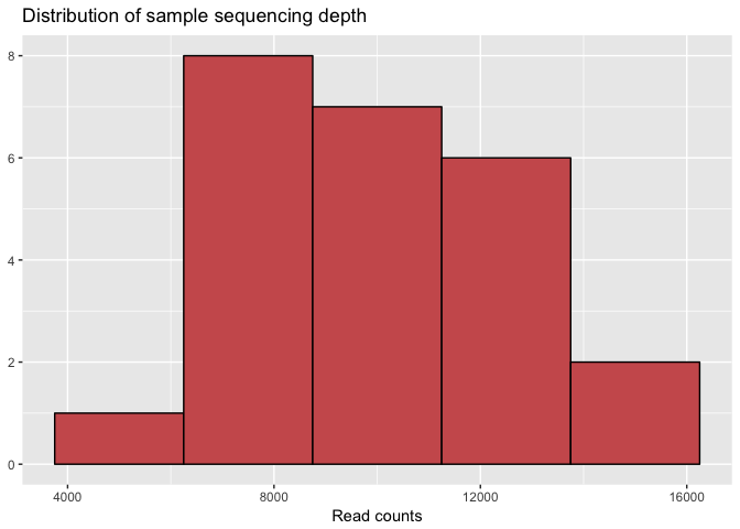
We want to check the distribution of read counts for each sample, to make sure we don’t have any outliers in terms of sequencing depth.
# We can use the `sample_sums()` function of phyloseq to add up total read counts for each sample.
sample_sum_df <- data.frame(sum = sample_sums(physeq))

# Histogram of sample read counts
ggplot(sample_sum_df, aes(x = sum)) +
  geom_histogram(color = "black", fill = "indianred", binwidth = 2500) +
  ggtitle("Distribution of sample sequencing depth") +
  xlab("Read counts") +
  theme(axis.title.y = element_blank())
Diversity Analysis
A basic question that nearly all microbial ecology studies seek to answer is ‘do the microbial communities differ between my treatments?’. The following sections will demonstrate how to perform basic analysis of alpha and beta diversity.
Check Alpha Diversity of Samples
A simple check of ‘how many unique observations are in each sample type’ can be useful for some studies. We will first plot different alpha diversty metrics, then perform an ANOVA on the unique observed sequences.
# Originally, the "Age variable was read as numerical, while I want it to be categorical. I use the `as.factor()` function to do this."
sample_data(physeq)$Age <- as.factor(sample_data(physeq)$Age)

#Phyloseq contains the `plot_richness()` function to display multiple alpha diversity measures at once. You can modify the plots based on sample metadata as well.
plot_richness(physeq, x="Site", measures=c("Observed", "Shannon", "Simpson", "Chao1", "InvSimpson"), color="Age") +   theme_bw()
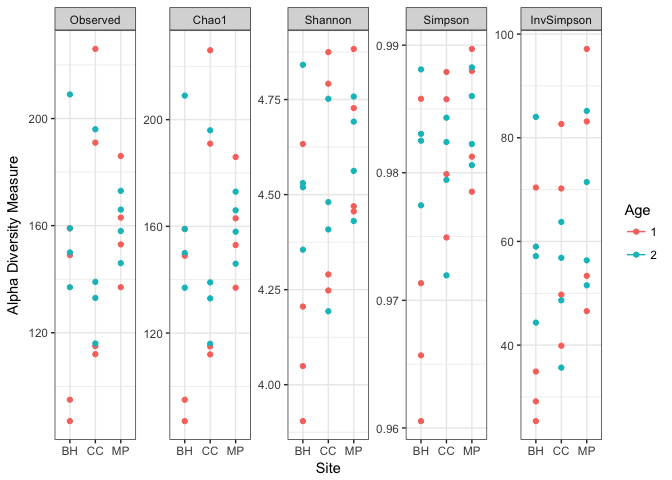
Now we can run an ANOVA on the ‘Observed’ diversity.
# First we will create a dataframe containing all diversity measures from above using the `estimate_richness()` function.
adiv <- estimate_richness(physeq, measures = c("Observed", "Shannon", "Simpson", "Chao1", "InvSimpson"))

# Then we can run an analysis of variance test using the `aov()` function.
summary(aov(adiv$Observed ~ physeq.m$Site))
##               Df Sum Sq Mean Sq F value Pr(>F)
## physeq.m$Site  2   1191   595.3   0.484  0.623
## Residuals     21  25806  1228.9
We can see here that there is no significant difference in the number of observed unique sequences by Site.
Calculate Distance Between Samples and Plot Ordinations
The distance function calculates distance between samples based on a given metric. We commonly use the Bray-Curtis metric, but wieghted and unweighted Unifrac can be used as well. A basic ordination plot is then created with the plot_ordination function.
# First, we normalize the sequence counts by converting from raw abundance to relative abundance. This removes any bias due to total sequence counts per sample.
pn = transform_sample_counts(physeq, function(x) 100 * x/sum(x))

# Next, we use the `distance()` function from phyloseq to generate a distance matrix from our phyloseq object. You can select from multiple methods; we will use Bray-Curtis
iDist <- distance(pn, method = "bray")

# Using the distance matrix created above, we now make an NMDS ordination using the `ordinate()` function.
pn.nmds = ordinate(pn,
                method = "NMDS",
                distance = iDist)

# Finally, we create an plot of the previous ordination using the `plot_ordination()` function. The `justDF` option is set to `TRUE`, which indicates that we only want the dataframe created with plot ordination to be returned, not a ggplot object.
plot.pn.nmds = plot_ordination(pn, pn.nmds, justDF = TRUE)
Using ggplot2, you can customize your plot with any metadata available in your sample_data file.
# Next we can display the figure using the `print(ggplot())` command, with any ggplot aesthetic arguments you want.
print(ggplot(plot.pn.nmds, aes(x = NMDS1, y = NMDS2, color = Site, shape = Age)) +
        geom_point( size = 4, alpha = 0.75))
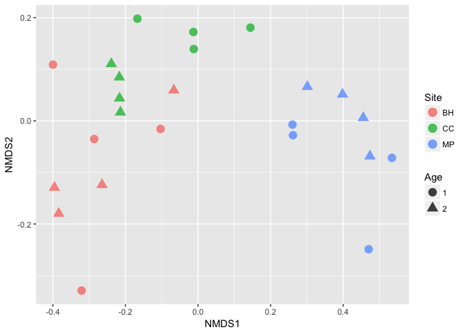
Simply observing what looks like a trend in an ordination is not the same as having statistical support, so we will now run a PERMANOVA test using the adonis() function in the vegan package.
library(vegan)
p.df = as(sample_data(pn), "data.frame")
p.d = distance(pn, method = "bray")
p.adonis = adonis(p.d ~ Site + Age + Site*Age, p.df)
p.adonis
##
## Call:
## adonis(formula = p.d ~ Site + Age + Site * Age, data = p.df)
##
## Permutation: free
## Number of permutations: 999
##
## Terms added sequentially (first to last)
##
##           Df SumsOfSqs MeanSqs F.Model      R2 Pr(>F)
## Site       2    2.2594 1.12968  7.5507 0.38795  0.001 ***
## Age        1    0.2723 0.27232  1.8202 0.04676  0.068 .
## Site:Age   2    0.5991 0.29956  2.0022 0.10287  0.025 *
## Residuals 18    2.6930 0.14961         0.46242
## Total     23    5.8239                 1.00000
## ---
## Signif. codes:  0 '***' 0.001 '**' 0.01 '*' 0.05 '.' 0.1 ' ' 1
Here, we can see that our communities significantly differ by Site, but not by Age. There is some interaction between the two variables as well. You can easily adjust the model to whatever metadata you desire.
Summarize Taxonomy at the Phylum Scale
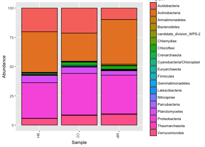
Sometimes you want to look at the relative abundance of major phyla in your samples, averaged over a particular metadata category.
# This normalization is redundant from before, but usefull if you want to just copy this chunk of code
pn = transform_sample_counts(physeq, function(x) 100 * x/sum(x))

# Here we use the `tax_glom()` function from phyloseq to collapse our OTU table at the Phylum level. This takes all OTUs under a given phylum and combines them, adding up the total sequence counts.
phylum = tax_glom(pn, taxrank="Phylum")

# Next, we want to look at just the average community by Site, not each individual sample. We will use the `merge_samples()` function to do this. You can use any categorical metadata variable for ths merge.
pm  = merge_samples(phylum, "Site")

# Phyloseq does some odd things with sample names when you merge, so this next line of code makes sure that everything will be labelled correctly for our figures.
sample_data(pm)$DeRep <- levels(sample_data(pm)$Sample)

# Again, we make a sample_data dataframe for future reference
pm.m = pm %>% sample_data

# Since each 'sample' in this new object is an agglomerate sample, we need to re-normalize our sequence counts for each OTU.
pm = transform_sample_counts(pm, function(x) 100 * x/sum(x))

# Finally, we can use the `plot_bar()` function to display our barchart.
plot_bar(pm, "Sample", fill = "Phylum")
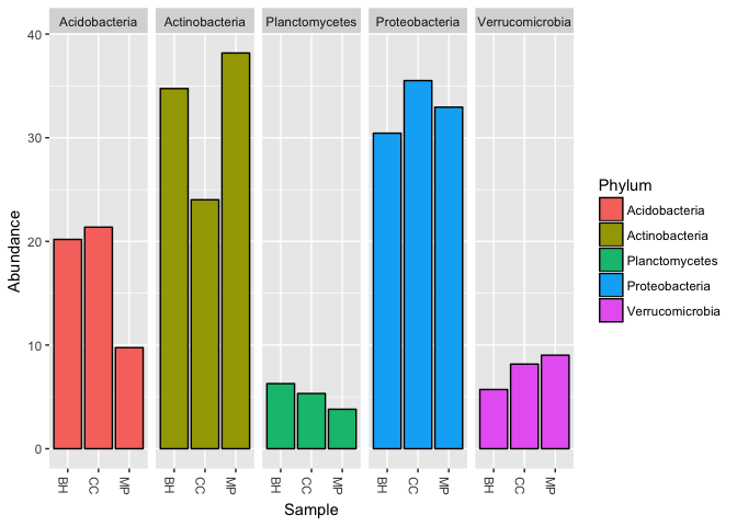
An alternative to the stacked barchart is to use the facet function of ggplot.
# Here, we will take a look at the top 5 most abundant phyla using the a faceted plot.

# First, create a list of the top 5 phyla
trimlist = names(sort(taxa_sums(pm), TRUE)[1:5])

# Then we will use the `prune_taxa()` function to select only those top 5 phyla
pm.5 = prune_taxa(trimlist, pm)

# Finally, we can plot the abundance of those phyla using the `facet_grid` argument for `plot_bar()`
plot_bar(pm.5, "Sample", fill = "Phylum", facet_grid = ~Phylum)
Differential Abundance Testing
After determining that our microbial communities significantly differ by Site, we might be interested in which unique sequences differ in abundance between our Sites. We will use the DESeq2 package for this analysis.
Set Up Dataframes and Run DESeq2
DESeq2 is an R package originally written to perform analyses of differential expression for RNA-Seq experiments. Fortunately, the methods used for those analysis are the same we need to perform analyses of differential abundnace for our community data. DESeq2 can only work with two conditions at a time, and since we have 3 sites, we will need to create a new phyloseq object with one site removed. You can perform this analysis on each of the three site pairings if you wish.
# Create a new `phyloseq` object with only the BH and MP sites.
mb = subset_samples(physeq, Site == "MP" | Site == "BH") %>%
                      filter_taxa(function(x) sum(x) > 0, TRUE)

# Next, we need to check the order of our Site levels. DESeq2 takes the first level as the 'Control' and the second level as the 'Treatment', and this is needed for downstream interpretation of results.
head(sample_data(mb)$Site)
## [1] BH BH BH BH BH BH
## Levels: BH MP
# Now we can prepare the DESeq2 object and run our analysis.
library(DESeq2)

# First, we will convert the sequence count data from our phyloseq object into the proper format for DESeq2
mb.dds <- phyloseq_to_deseq2(mb, ~ Site)

# Next we need to estimate the size factors for our sequences
gm_mean = function(x, na.rm=TRUE){
    exp(sum(log(x[x > 0]), na.rm=na.rm) / length(x))
}
geoMeans = apply(counts(mb.dds), 1, gm_mean)
mb.dds = estimateSizeFactors(mb.dds, geoMeans = geoMeans)

# Finally, we can run the core DESeq2 algorithm
mb.dds = DESeq(mb.dds, fitType="local")
Format Results Table
Next, we will trim our results and take a look at those OTUs that showed a significant difference in abundance between our two sites.
# Create a new dataframe from the results of our DESeq2 run
mb.res = results(mb.dds)

# Reorder the sequences by their adjusted p-values
mb.res = mb.res[order(mb.res$padj, na.last=NA), ]

# Set your alpha for testing significance, and filter out non-significant results
alpha = 0.01
mb.sigtab = mb.res[(mb.res$padj < alpha), ]

# Add taxonomy information to each sequence
mb.sigtab = cbind(as(mb.sigtab, "data.frame"), as(tax_table(mb)[rownames(mb.sigtab), ], "matrix"))
head(mb.sigtab)
##        baseMean log2FoldChange    lfcSE      stat       pvalue
## OTU.24 6.686493       9.783456 1.069434  9.148253 5.786182e-20
## OTU.12 4.985300      -9.044197 1.127915 -8.018507 1.070383e-15
## OTU.50 3.893791       8.965181 1.177931  7.610957 2.720744e-14
## OTU.52 4.273686       9.081006 1.198890  7.574512 3.604797e-14
## OTU.72 3.304191       8.680833 1.269083  6.840241 7.905980e-12
## OTU.85 2.997141       8.559756 1.246743  6.865696 6.616774e-12
##                padj  Kingdom          Phylum               Class
## OTU.24 1.556483e-17 Bacteria  Proteobacteria Alphaproteobacteria
## OTU.12 1.439665e-13 Bacteria            <NA>                <NA>
## OTU.50 2.424226e-12 Bacteria Verrucomicrobia      Spartobacteria
## OTU.52 2.424226e-12 Bacteria  Actinobacteria      Actinobacteria
## OTU.72 3.544514e-10 Bacteria Verrucomicrobia      Spartobacteria
## OTU.85 3.544514e-10 Bacteria  Actinobacteria      Actinobacteria
##                   Order             Family        Genus
## OTU.24      Rhizobiales  Xanthobacteraceae Pseudolabrys
## OTU.12             <NA>               <NA>         <NA>
## OTU.50             <NA>               <NA>         <NA>
## OTU.52  Actinomycetales Micromonosporaceae         <NA>
## OTU.72             <NA>               <NA>         <NA>
## OTU.85 Acidimicrobiales               <NA>         <NA>
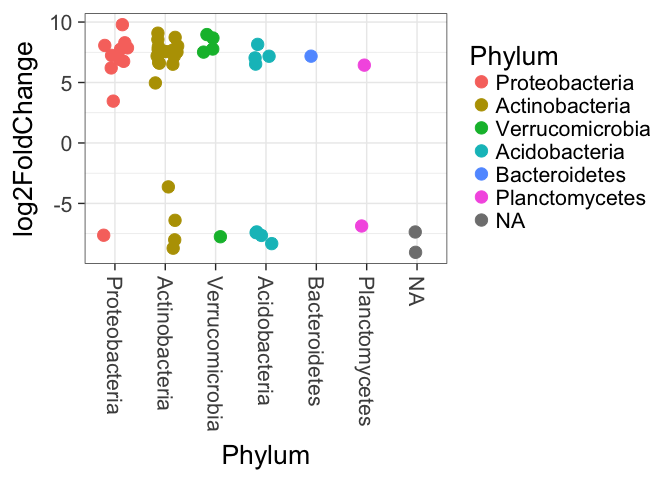
Plot DESeq2 Results
Now we can graph our results from DESeq2. In the plot below, each individual point represents a unique sequence from our dataset that was found to be significantly higher in abundance in one sample type or the other. The log2 fold change value represents the magnitude of that difference in abundance. The higher the value, the greater the difference in abundance in one sample type compared to the other.
At this point we need to consult the information we gathered earlier on the levels of our Site variable. In DESeq2, any sequence that is more abundant in the ‘Control’ variable will have a negative log2 fold change value, and any sequence more abundant in the ‘Treatment’ variable will have a positive value. In our case, sequences more abundant in the ‘BH’ site will have negative values, and those more abundant in ‘MP’ values will have a positive value.
# Set ggplot2 options
theme_set(theme_bw(base_size = 20))
scale_fill_discrete <- function(palname = "Set1", ...) {
    scale_fill_brewer(palette = palname, ...)
}
# Rearrange the order of our OTUs by Phylum.
x = tapply(mb.sigtab$log2FoldChange, mb.sigtab$Phylum, function(x) max(x))
x = sort(x, TRUE)
mb.sigtab$Phylum = factor(as.character(mb.sigtab$Phylum), levels=names(x))

# Create and display the plot
p = ggplot(mb.sigtab, aes(x=Phylum, y=log2FoldChange, color=Phylum)) + geom_jitter(size=4, width=0.25) +
  theme(axis.text.x = element_text(angle = -90, hjust = 0, vjust=0.5))
p
References
Sequencing Primers
Kozich JJ, Westcott SL, Baxter NT, Highlander SK, Schloss PD. 2013. Development of a dual-index sequencing strategy and curation pipeline for analyzing amplicon sequence data on the MiSeq Illumina sequencing platform. Appl Environ Microbiol 79(17): 5112-5120
DADA2
Callahan BJ, McMurdie PJ, Rosen MJ, Han AW, Johnson AJA, Holmes SP. 2016. DADA2: High-resolution sample inference from Illumina amplicon data. Nature Methods 13, 581-583
Phyloseq
McMurdie and Holmes (2013) phyloseq: An R Package for Reproducible Interactive Analysis and Graphics of Microbiome Census Data. PLoS ONE. 8(4):e61217
DESeq2
Love MI, Huber W and Anders S (2014). “Moderated estimation of fold change and dispersion for RNA-seq data with DESeq2.” Genome Biology, 15, pp. 550
Vegan
Oksanen J, Blanchet FG, Friendly M, Kindt R, Legendre P, McGlinn D, Minchin PR, O’Hara RB, Simpson GL, Solymos P, Stevens MHH, Szoecs E, and Wagner H. 2016. vegan: Community Ecology Package. R package version 2.4-1.